
- Engineering
Jitter buffers for conversation: how much waiting is too much?
Compare receiver waiting and late audio using controlled jitter replay, raw counters, and explicit conversation-quality boundaries.
- Author
 Udit Goenka
- Editorial date
- Reading time
- 25 min
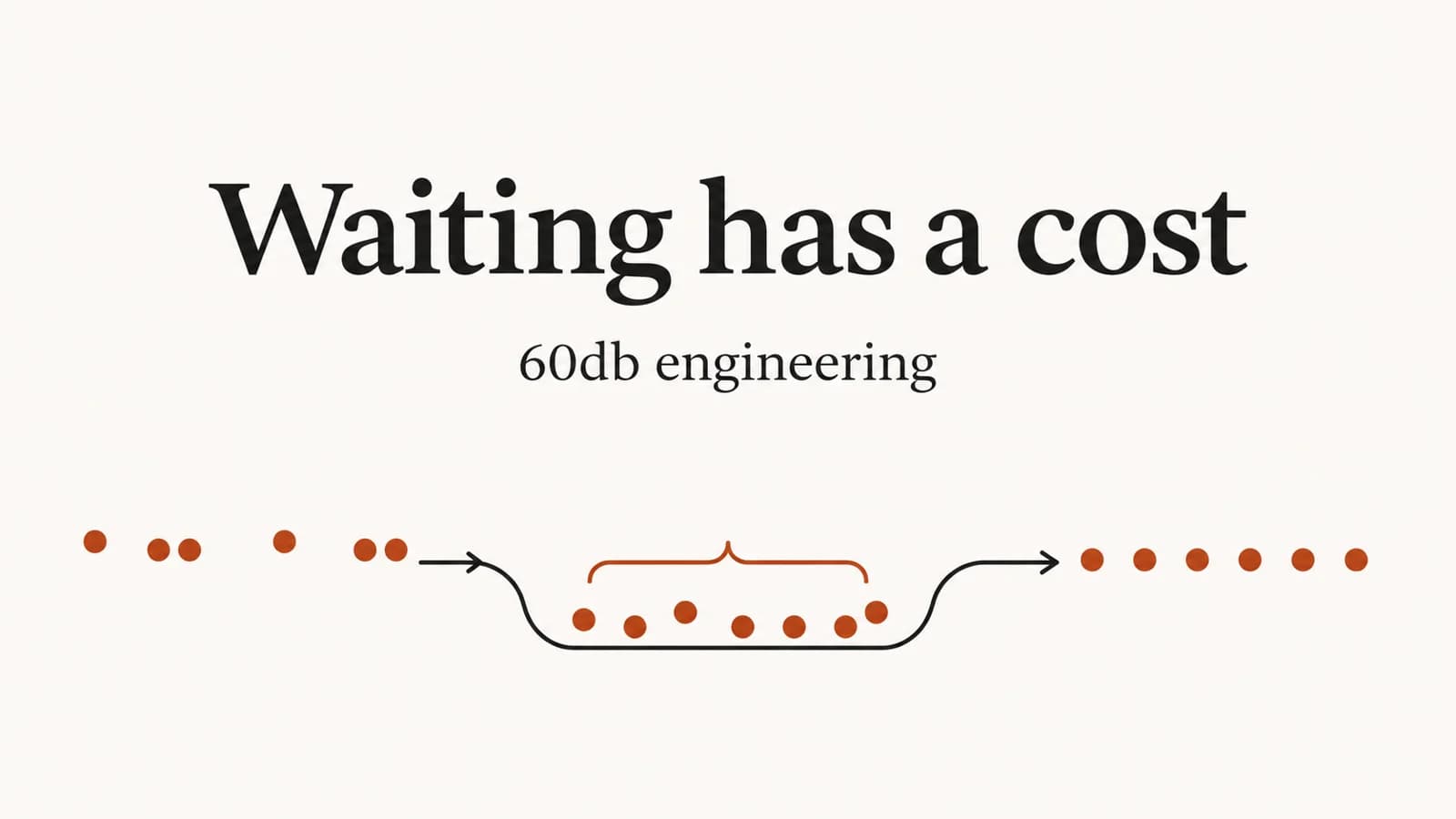
TL;DR: A conversation jitter buffer trades additional receiver waiting for a chance to play irregularly arriving audio on time. Compare policies on the same arrival trace, preserve late and missing outcomes separately, and measure interval buffer delay from the original counters rather than treating RTP jitter or a requested target as end-to-end latency.
The voice sounds smooth, but each reply reaches the caller after the moment it would have been useful. Increasing buffering repaired audible gaps while adding another kind of failure: the conversation now waits behind old speech.
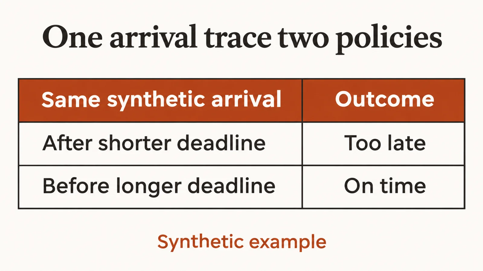
The opposite setting can fail too. A very short receiver deadline can make packets unusable even when they eventually arrive, leaving the decoder to fill gaps that the network did not permanently lose.
Start with the playout deadline for one declared receiver boundary. Ask which arrivals would meet that deadline and how much extra waiting the accepted media would experience before choosing a browser target or production policy.
The transport boundary guide explains why the answer depends on the actual media path. This article adds a deterministic replay, a raw-counter worksheet, and a conversation-focused evaluation method.
Every fixture is synthetic. The program does not implement a browser jitter buffer, decode a codec, measure a physical speaker, or describe private 60db Agent behavior.
Table of contents
- Define the receiver waiting boundary
- Separate jitter from buffer delay
- Construct a controlled arrival trace
- Run replay and counter fixtures
- Interpret interval evidence correctly
- Compare policies without hiding failures
- Protect interruption and current intent
- Review the actual listening outcome
- Qualify browser and device behavior
- Build a useful operating report
- Keep the denominator attached to the question
- Design a controlled trial around the replay
- Frequently asked questions
- Begin with a shared trace
Define the receiver waiting boundary
A jitter buffer holds irregularly arriving media so the receiver can supply a steadier playback sequence. Its useful operating point depends on the arrival pattern, decoder behavior, deadline policy, and the interaction the listener is trying to complete.
Define which waiting you intend to measure. Receiver buffer waiting is different from capture accumulation, application queue age, network transit, decoding work, audio-device scheduling, and the caller's opportunity to hear the result.
The latency measurement guide keeps those boundaries separate. A change to one receiver setting should be evaluated at that boundary before being credited with an improvement in the entire conversation.
A packet can reach the receiver before its deadline and still spend time waiting there. Another packet can arrive after its deadline and contribute nothing to the played original media, even though a network trace eventually shows successful delivery.
That distinction is the first useful diagnostic. If the caller hears gaps while network delivery counters look acceptable, investigate deadlines and late discards instead of assuming the microphone or recognizer dropped the words.
For conversational audio, more waiting can reduce some audible damage while making interruption recovery worse. The caller may correct a value while the receiver is still playing a sentence that was generated for an older question.
A response deadline is a product decision as well as a media decision. A public explanation that remains useful after a short pause differs from an instruction whose timing depends on what the caller is doing now.
Do not choose a universal maximum from a diagram or an old forum reply. Establish the task's acceptable behavior, replay representative arrival traces, and inspect the trade-off that the tested policy produces.
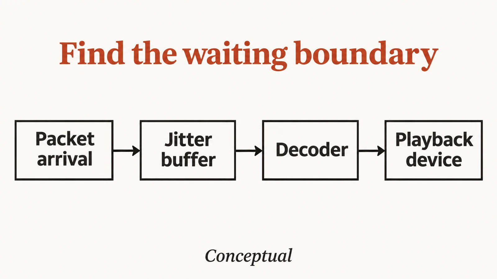
The figure identifies a conceptual processing boundary. Real implementations can combine buffering and decoding internally, so its boxes are measurement responsibilities rather than an assertion about a browser's private pipeline.
Separate jitter from buffer delay
RTP interarrival jitter describes variation according to the estimator defined in RFC 3550. It does not directly state how long an application should buffer or how long the caller waited for a useful answer.
A receiver's buffering policy can react to changing conditions. The current reported jitter and the accumulated waiting experienced by samples can move differently after a short disturbance or a policy change.
The WebRTC statistics specification defines cumulative jitter-buffer delay and emitted counts. Its metric describes its own ingest-to-emission boundary, leaving later audio-device waiting outside that observation.
Use the statistics document's units. jitterBufferDelay accumulates seconds associated with emitted media, while jitterBufferEmittedCount counts emitted samples for audio; dividing appropriate counter deltas yields an interval mean in seconds per emitted sample's buffer stay.
A cumulative ratio answers a different question from an interval ratio. Reading the lifetime average after a recent disturbance can dilute the very period you are trying to diagnose.
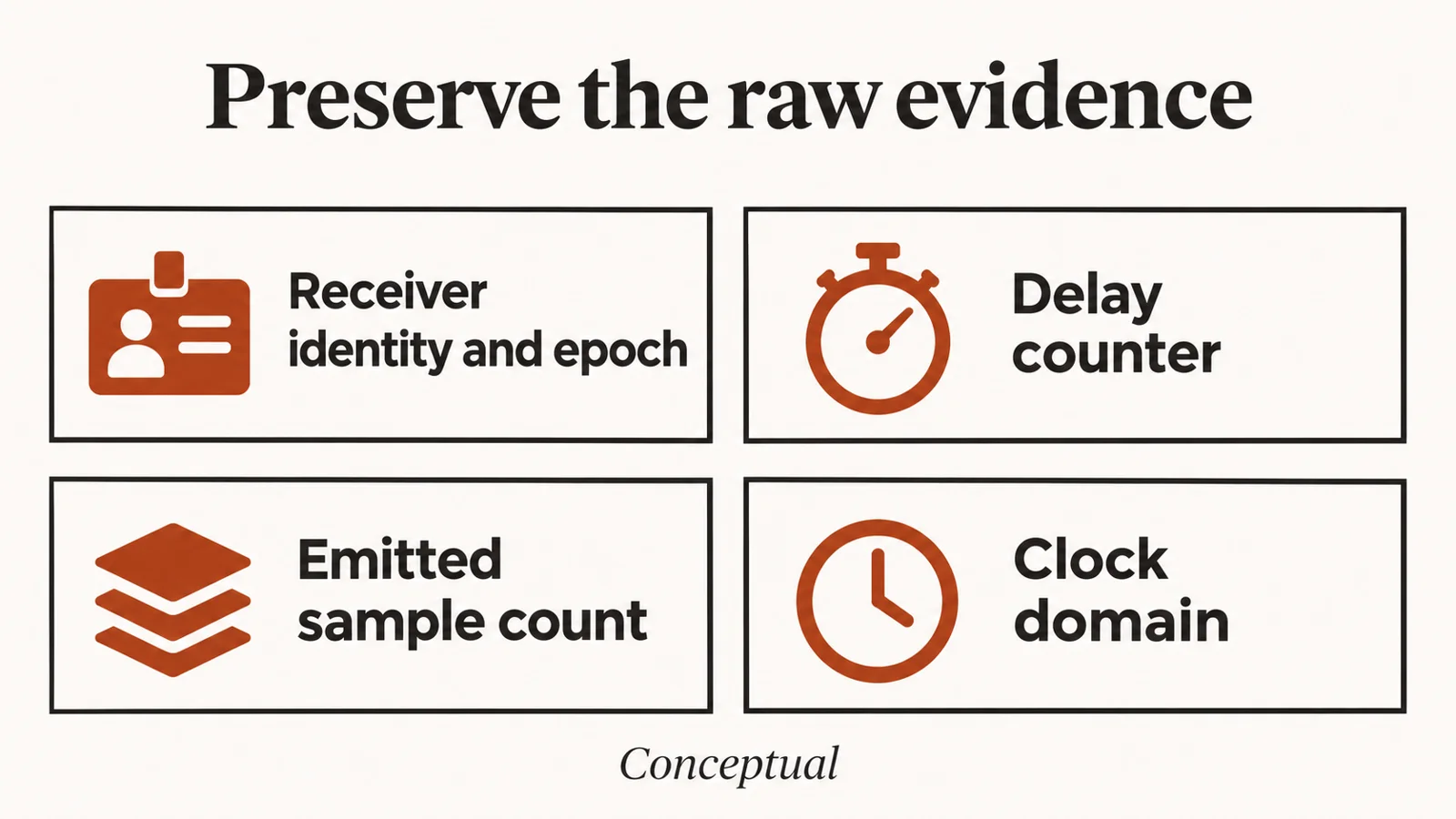
Preserve the original cumulative values before calculating a delta. A dashboard that stores only a derived millisecond value cannot reconstruct which receiver, emitted population, or reset produced that value.
The voice observability guide provides the event-boundary approach. Keep stream identity, timestamp, clock domain, counters, and availability alongside the derived result.
Do not replace unavailable data with zero. A zero counter can be a valid observation, while an absent field means the metric was not supplied and cannot support the same calculation.
An old developer discussion asks what reception boundary the delay statistic uses. It is useful historical context for the question, while the current specification and actual receiver implementation own the answer for your tested version.
Avoid subtracting an unrelated round-trip time from buffer delay and calling the remainder a measured local defect. The quantities refer to different boundaries and may lack the relationship required for that arithmetic.
Construct a controlled arrival trace
A controlled trace needs expected media identity as well as observed arrivals. Without the expected population, the replay cannot distinguish a packet that never arrived from one that was never part of the fixture.
The reference uses a fixed packet duration and one synthetic clock. Sequence position determines the media schedule, and a chosen startup offset determines each packet's playout deadline.
This is a small fixed-policy model. It intentionally omits adaptive delay control, packet loss concealment, decoder state, transport feedback, and device scheduling so its results have a narrow interpretation.
Keep the actual arrival sequence in the fixture. A random seed can help generate a trace, but retaining the generated identities and times makes the comparison reproducible even if a library's random implementation changes.
A repeated identical arrival is a duplicate observation. A second arrival that reuses the same packet identity with changed data is a conflict under this fixture contract, so the example rejects it instead of silently choosing whichever value is convenient.
Real RTP sequence numbers can wrap, and receivers can restart. A production adapter needs an extended sequence and stream identity rule; the compact replay accepts a finite already-normalized population rather than pretending to solve those adapter concerns.
The chunk-size guide explains why packet count and audio duration are not interchangeable. Fixed duration makes the sample calculation simple here; variable-duration traces need duration-aware accounting.
A trace also needs a declared deadline comparator. The example accepts arrival exactly at the deadline and treats later arrivals as too late, which makes its boundary tests deterministic.
Do not attach a human listening score to this replay output. It establishes deadline eligibility and waiting in the stated model, while the actual codec and listener can experience the same trace differently.
Run replay and counter fixtures
Save this complete fence as jitter_replay.py and run Python 3.11 or later. It uses only the standard library and prints a passing fixture message after checking replay boundaries and counter-delta validity.
The trusted input is a normalized synthetic trace plus receiver statistics from one declared identity and clock. The adapter owns real packet parsing, codec behavior, browser compatibility, counter capture, and physical playback evidence.
import math
from dataclasses import dataclass, replace


def finite(value):
    return type(value) in (int, float) and math.isfinite(value)


def replay(count, frame_ms, startup_ms, arrivals):
    if type(count) is not int or count < 1:
        raise ValueError("positive packet population required")
    if not finite(frame_ms) or frame_ms <= 0:
        raise ValueError("positive frame duration required")
    if not finite(startup_ms) or startup_ms < 0:
        raise ValueError("nonnegative startup required")
    observed = {}
    for sequence, arrival_ms in tuple(arrivals):
        if type(sequence) is not int or not 0 <= sequence < count:
            raise ValueError("unknown packet identity")
        if not finite(arrival_ms) or arrival_ms < 0:
            raise ValueError("invalid arrival time")
        if sequence in observed and observed[sequence] != arrival_ms:
            raise ValueError("conflicting duplicate")
        observed[sequence] = arrival_ms
    rows = []
    for sequence in range(count):
        deadline = sequence * frame_ms + startup_ms
        arrival = observed.get(sequence)
        outcome = ("missing" if arrival is None else
                   "on_time" if arrival <= deadline else "too_late")
        wait = deadline - arrival if outcome == "on_time" else None
        rows.append((sequence, outcome, wait))
    return tuple(rows)


@dataclass(frozen=True)
class Sample:
    receiver: str
    clock: str
    observed_at: float
    delay_seconds: float | None
    emitted_count: int | None
    epoch: int = 0


def interval(before, after):
    if (before.receiver, before.clock, before.epoch) != (after.receiver, after.clock, after.epoch):
        return "identity_changed", None
    if not all(finite(s.observed_at) for s in (before, after)):
        return "invalid_time", None
    if after.observed_at <= before.observed_at:
        return "nonincreasing_time", None
    for sample in (before, after):
        if sample.delay_seconds is None or sample.emitted_count is None:
            return "unavailable", None
        if (not finite(sample.delay_seconds) or sample.delay_seconds < 0
                or type(sample.emitted_count) is not int
                or sample.emitted_count < 0):
            return "invalid_counter", None
    delay = after.delay_seconds - before.delay_seconds
    emitted = after.emitted_count - before.emitted_count
    if delay < 0 or emitted < 0:
        return "counter_reset", None
    if emitted == 0:
        return "no_emitted_samples", None
    return "measured_interval", delay / emitted


def tests():
    arrivals = [(0, 0), (1, 25), (2, 100)]
    short = replay(4, 20, 10, arrivals)
    assert short == ((0, "on_time", 10), (1, "on_time", 5),
                     (2, "too_late", None), (3, "missing", None))
    assert replay(4, 20, 10, reversed(arrivals)) == short
    assert replay(1, 20, 10, [(0, 10), (0, 10)]) == ((0, "on_time", 0),)
    assert replay(1, 20, 10, [(0, 11)])[0][1] == "too_late"
    assert replay(1, 20, 0, [])[0][1] == "missing"
    before = Sample("receiver-a", "local-monotonic", 0, 0, 0)
    after = Sample("receiver-a", "local-monotonic", 1, 2, 100)
    assert interval(before, after) == ("measured_interval", 0.02)
    assert interval(before, replace(after, delay_seconds=0)) == ("measured_interval", 0)
    cases = [(replace(after, epoch=1), "identity_changed"),
             (replace(after, receiver="receiver-b"), "identity_changed"),
             (replace(after, clock="other"), "identity_changed"),
             (replace(after, observed_at=0), "nonincreasing_time"),
             (replace(after, delay_seconds=None), "unavailable"),
             (replace(after, emitted_count=0), "no_emitted_samples"),
             (replace(after, delay_seconds=float("nan")), "invalid_counter")]
    for sample, expected in cases:
        assert interval(before, sample) == (expected, None)
    assert interval(after, replace(after, observed_at=2, emitted_count=1)) == ("counter_reset", None)
    for args in [(0, 20, 0, []), (1, 0, 0, []), (1, 20, -1, []),
                 (1, 20, 0, [(1, 0)]), (1, 20, 0, [(0, float("nan"))]),
                 (1, 20, 0, [(0, 0), (0, 1)])]:
        try:
            replay(*args)
            raise AssertionError("invalid trace accepted")
        except ValueError:
            pass
    print("synthetic jitter replay and counter fixtures passed")


if __name__ == "__main__":
    tests()
The synthetic numeric settings are fixture inputs, not recommended buffering values. The program's interval result is derived from supplied synthetic counters and does not represent a measured browser or caller population.
The replay returns immutable result tuples. It copies arrival observations into its own dictionary and does not retain a mutable caller-owned container as an approved media schedule.
Interpret interval evidence correctly
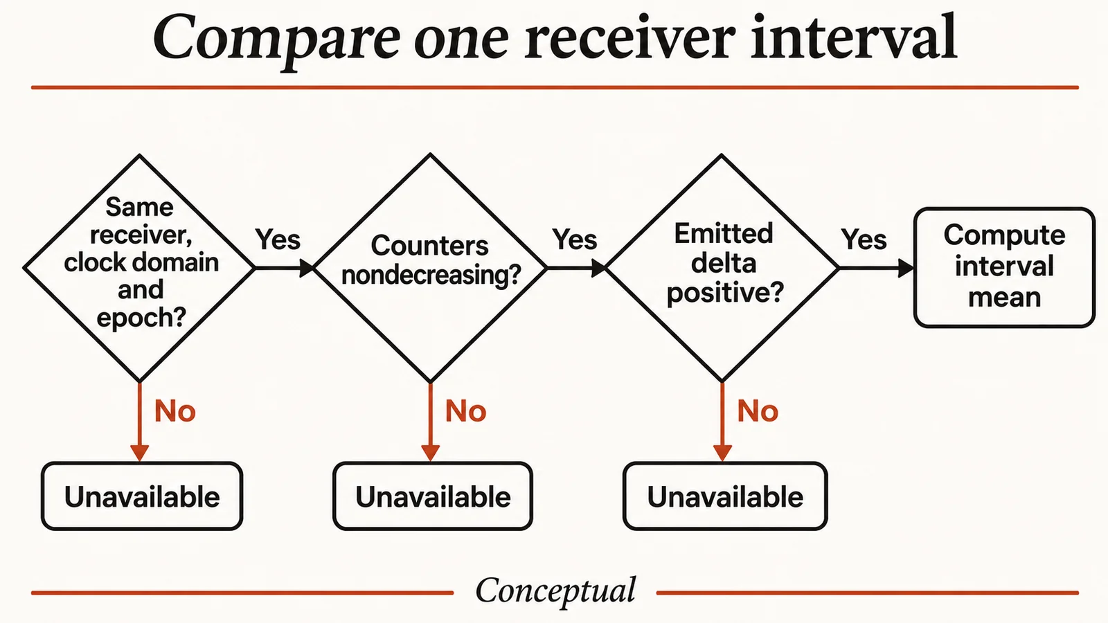
The interval calculation needs a stable receiver identity and a monotonically advancing observation boundary. A new stream or receiver epoch, including a restart that reuses the same SSRC and apparent counter values, should start another baseline rather than producing a negative or inflated delay value.
A counter can increase while the latest sample's target changes. The ratio describes the emitted population over the interval, so it should not be labeled as the instantaneous current target.
When combining intervals, add their delay deltas and emitted deltas before dividing. Averaging interval means without their emitted weights gives an interval with very few samples the same influence as a much larger population.
Keep that aggregation within the declared receiver cohort and measurement contract. If the analysis intentionally combines receivers, retain their individual raw inputs and state the population rather than presenting the sum as one uninterrupted stream.
A zero emitted delta has no emitted population for the mean. The reference returns a typed unavailable result even when the delay counter also stayed zero, preserving the difference between no observation and a measured zero stay.
A decreasing counter invalidates the interval. Do not clamp the delta to zero, since that turns a restart or identity mismatch into a plausible measurement and can hide a broken collection path.
The audio backpressure guide covers another age measure: time already spent waiting in an application queue. It can reveal old output even while the receiver's own buffer statistics remain modest.
A receiver buffer statistic and a local queue statistic can both be correct while describing different populations. Join their event identities and scopes before deciding which component introduced the delay.
Keep unavailable fields in the report. A browser that omits a statistic has not established that the corresponding delay or concealment was zero.
Compare policies without hiding failures
Compare policy candidates on the same expected media schedule and arrival observations. Changing the trace while changing the policy prevents the replay from identifying which difference caused the outcome.
For each candidate, retain on-time, too-late and missing counts, the represented duration, and the waiting of accepted media. Report the chosen denominator whenever a ratio appears.
A larger startup offset can make additional arrivals meet the deadline in the fixed model. It also changes the scheduled output time, so a report that shows only reduced late loss leaves out part of the decision.
The following table compares evidence types. A check means the method establishes that property under its stated scope; a cross means another observation is needed.
| Criterion | Arrival replay | Receiver counter intervals | Consented listening trial |
|---|---|---|---|
| Exact synthetic deadline outcomes | ✓ Deterministic fixture | ✗ Aggregate only | ✗ Needs trace alignment |
| Receiver sample-weighted waiting | ✗ Model only | ✓ Supported raw counters | ✗ Not directly observed |
| Device audibility | ✗ No | ✗ No | ✓ At declared acoustic setup |
| Caller comprehension | ✗ No | ✗ No | ✗ Requires task observation |
| General production recommendation | ✗ No | ✗ No | ✗ Needs representative qualification |
The burst-loss guide adds another dimension. Equal average loss rates can hide very different gap sequences, and a buffer cannot turn every missing run into timely original media.
The recovery mechanism guide distinguishes actual recovered payload from locally synthesized replacement audio. Smooth output alone does not tell you which mechanism supplied the samples.
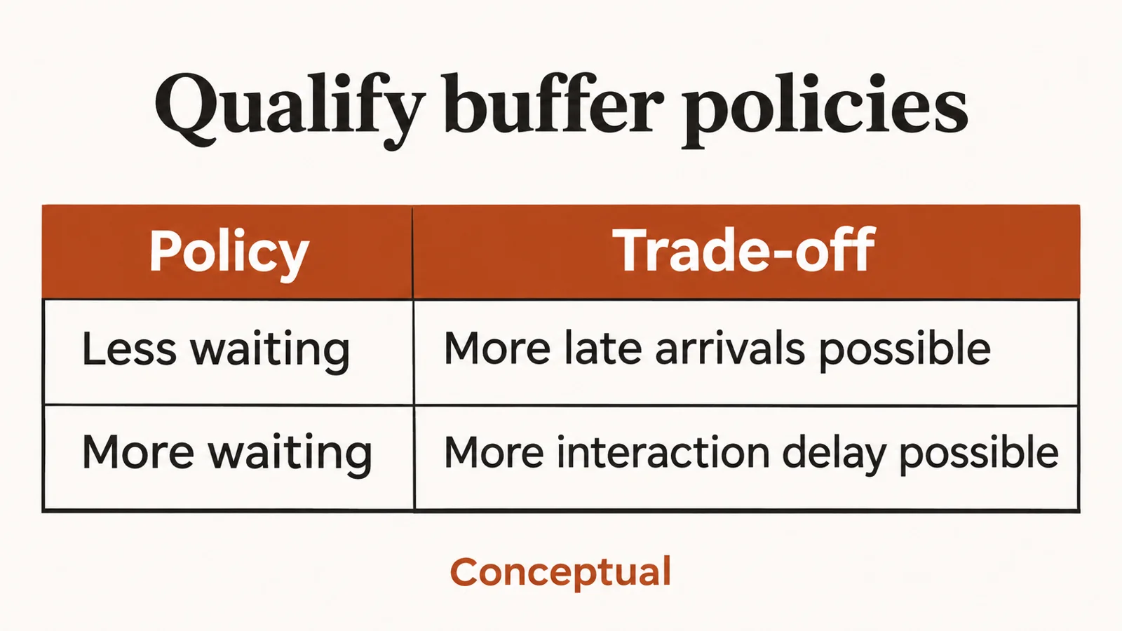
Keep failed and incomplete trials in the report. Removing runs that could not sustain playback can make an aggressive policy appear faster by excluding the requests it failed to serve.
Protect interruption and current intent
A playout policy does not own the conversation's accepted facts. When the caller corrects a material value, prepared old speech must lose authority even if its arrival timing remains within the media deadline.
The interruption-safe output guide provides the generation boundary. The buffer's smoothness objective should operate inside that boundary rather than treating every available packet as permanently playable.
Keep a response generation on application-owned media and a separate transport or receiver identity where the connection lifecycle differs. Reconnecting should not make an old generation current simply because a new socket can send its bytes.
The network-change recovery guide develops that case. It treats connectivity, response validity and business operation state as separate facts.
After a wait, compare identity before applying expiry side effects. An old held item can be both stale and expired, but rejecting it must not cancel the newer response that replaced it.
If the application clears old output, respect the actual receiver contract. A local queue deletion cannot retract media already accepted downstream or sound the listener already heard.
The playback acknowledgment guide explains those observations. They establish supported delivery boundaries, leaving hearing and comprehension to their own evidence.
Review the actual listening outcome
A deadline replay can guide a controlled experiment, but it cannot tell whether a listener understood a critical name, negation, or instruction. Use a real decoder adapter and a safe listening task to evaluate that next boundary.
Freeze the source audio and impairment trace across candidates. Record codec configuration, channel, packetization, receiver version, device setup, and whether the listener was asked to identify a particular critical field.
The retrieval-to-speech review guide supplies an answer-level rubric. An audio sequence can be pleasant and still fail because a required condition was delayed, obscured, or separated from its claim.
Test interruption points as well as uninterrupted playback. Ask whether obsolete speech stops at the supported boundary and whether the next answer reflects the current question without forcing unnecessary repetition.
The outcome metrics guide keeps task success separate from intermediate quality signals. Report a critical-field error even when the average signal sounds acceptable to a casual reviewer.
Do not label synthetic concealment as recovered original speech. The Opus specification provides the codec context; actual decode and listening results need the tested implementation and workload.
Keep the test corpus private where real speech requires it. Synthetic fixtures can cover deterministic ordering, while consented representative speech can expose pronunciation and task effects that an artificial signal misses.
Qualify browser and device behavior
A browser API setting is a request under that API's contract. MDN's jitterBufferTarget documentation is a useful compatibility and semantics reference, but actual achieved behavior must be observed for the tested browser version.
Feature-detect before applying a setting. Record the requested value separately from observed counter deltas, and do not silently substitute an unsupported field with a fake successful result.
A historical developer question asks about jitter-buffer sizing in Chrome. Its age matters: use it to motivate the trade-off, not to assert what a current browser can configure.
The mobile browser guide identifies lifecycle and device conditions worth separating. A route change, background transition or audio-device switch can alter the evidence without implying the buffering algorithm alone is defective.
For an end-to-end network trial, use a controlled impairment tool. The netem manual documents supported delay and loss models and their limits; a later trial should isolate the test interface and restore its configuration afterward.
No network configuration is changed by the published Python example. Its fixture clock is local and synthetic, so passing it does not prove a real carrier or browser honors the modeled schedule.
Build a useful operating report
A useful report starts with the decision and the tested boundary. State whether the candidate changed requested receiver buffering, an application deadline, or another parameter, then attach the exact trace and raw observations used to evaluate it.
Keep configuration and observation separate. A requested target belongs in configuration; achieved interval waiting belongs in evidence; listener task outcome belongs in the evaluation record.
The regression testing guide explains how to preserve a discovered failure as a fixture. Keep the short burst or interruption ordering that caused the problem rather than replacing it with a smooth average trace.
Report the operational cost too. The cost-per-success guide shows why extra retries and repeated calls can outweigh a narrow gain in one media metric.
State what remains unknown. A passing fixed replay does not establish the correct adaptive policy, and a successful desktop listening trial does not establish performance across mobile routes or all listener needs.
Keep the denominator attached to the question
A packet population, an emitted-sample population, and a caller-task population answer different questions. Keep all of them visible when comparing a buffering change, because an improvement under one denominator can coexist with a failure under another.
The replay's expected packet count is fixed before the arrivals are inspected. That prevents a packet that never arrived from disappearing from the experiment simply because there was no receiver event to count.
Its on-time count includes only arrivals that meet the declared deadline. Waiting is calculated for that accepted population, so the report must also show how much of the expected population was excluded as missing or too late.
A candidate that accepts fewer packets can show a smaller mean wait among its survivors. That arithmetic is valid for the accepted subset and misleading if presented as the whole experience without the excluded outcomes.
The receiver statistics use a different population: emitted samples under the specification's boundary. A packet-level replay with fixed durations is useful for reasoning, but it cannot be substituted for the receiver's actual sample accounting when decoder behavior changes the emitted sequence.
Keep packet duration explicit even when every packet in the initial fixture has the same duration. A future experiment that changes packetization can otherwise preserve the same packet counts while changing the amount of damaged or buffered audio.
A variable-duration adapter should retain media duration per identity. It can then report represented missing duration and accepted duration without assuming every lost network packet carried an equal portion of speech.
The distinction matters for silence and discontinuous transmission too. An interval with no expected speech packets is different from an interval whose expected speech packets all failed to arrive.
Do not fill missing expected-media knowledge with zero loss. If the adapter cannot establish the sent or expected population, report the available observations and mark the missing denominator rather than inventing a complete delivery ratio.
Keep send-side and receive-side observations separate. A sender can record that it created a packet without proving local transport acceptance, network delivery, receiver admission, or acoustic output.
If the investigation needs an end-to-end count, join identities across those observations under a declared loss and retry policy. Packet duplication, retransmission, and redundant payload can make raw network packet counts differ from unique useful media identities.
The recovery mechanism comparison helps keep that accounting honest. Recovering an earlier unit from redundancy is not the same as receiving another original packet, and concealment can add output samples without supplying the missing original content.
For interval aggregation, retain both deltas alongside each computed mean. If one interval emits little audio and another emits much more, weighting by emitted count gives the combined sample-level result; an unweighted average answers the mean-of-intervals question instead.
Both calculations can be useful if named correctly. The failure is reporting one while implying the population and weighting of the other.
State the treatment of invalid intervals before looking at results. Receiver changes, counter resets, unavailable fields, and nonincreasing timestamps should remain counted as collection outcomes rather than vanishing from a clean-looking average.
A collection defect can correlate with the worst operating conditions. Dropping invalid intervals without showing their frequency may remove the exact route changes or overload periods the report needs to explain.
Keep the original raw observation sequence in a controlled diagnostic bundle. A table of rounded derived milliseconds cannot recover whether a reset occurred between two observations or whether a receiver identity was reused incorrectly.
For the caller-level outcome, define a task rather than a sound preference alone. A useful test can ask the listener to repeat a critical value, follow one harmless instruction, or identify whether the answer changed after a correction.
A task failure should remain visible even when the audio reviewer rated the stream as smooth. Smooth playback can preserve every sample of an answer that arrived too late or belonged to an obsolete question.
The spoken answer contract gives the response-level boundary. Keep required conditions with their claim so a buffering experiment does not accidentally reward an output policy that speaks the easy part first and delays the qualifying information.
When reporting a policy decision, name which denominators supported it. You may choose a setting that slightly increases receiver waiting because it preserves a critical field on the qualified workload, while still documenting the added recovery delay and the routes that remain unqualified.
That is a bounded engineering decision. It does not require a fabricated universal threshold, a single blended quality score, or a claim that the chosen setting is optimal for every conversation.
Design a controlled trial around the replay
Use the deterministic replay to identify a small set of schedules worth testing with a real media adapter. The most useful cases are those that separate candidate behavior, not a large pile of random traces that all produce the same outcome.
Begin with an undamaged baseline. It checks that the media representation, decoder, and playback path work before an impairment is introduced, preventing a format error from being misdiagnosed as a buffering trade-off.
Then introduce a short late-arrival episode with otherwise unchanged media. Keep the original expected schedule and record the actual arrivals so the adapter's observed behavior can be compared with the fixed model's prediction.
Add a missing-packet case independently. The buffer can wait for a late arrival under some policies, while no finite wait creates original data that never arrives, so those cases should not be combined into one generic poor-network scenario.
Add reordering without permanent loss. A receiver may have to place media back into its intended order, and the trace should reveal whether the chosen deadline leaves time for that recovery.
Add duplicates and conflicting identities to the input adapter's tests. A duplicate should not create another emitted population or extend generation history, and conflicting payload evidence should not be silently accepted under an existing identity.
Include a disturbance near the start and another after steady playback. An adaptive implementation may treat startup and ongoing playout differently, so a single initial burst is insufficient evidence for the entire call lifecycle.
The fixed reference does not adapt. Preserve that limitation when comparing it with a browser: differences can reveal assumptions to investigate, not automatically a browser defect.
For a physical listening trial, select a safe synthetic phrase with a critical field. Keep its canonical expected value outside the audio so reviewers can distinguish missing or altered content from a vague impression that the stream sounded unusual.
Use an interruption case that changes the accepted answer. Hold old media while the caller supplies the synthetic correction, then verify that the application invalidates controllable output and the recovery uses the corrected fact.
The post-interruption recovery guide distinguishes repeating a complete step from continuing an arbitrary tail. A buffering change should not force recovery to replay an outdated fragment just because that fragment is still available.
Include a sender stall separately from receiver jitter. A producer that stops generating data creates a different evidence pattern from a healthy producer whose packets arrive irregularly, and adding receiver delay may mask the symptom without addressing the cause.
The WebSocket stall diagnosis guide helps separate ordered-delivery waiting from application scheduling. If the tested WebRTC path uses a relay transport, record that route rather than assuming it behaves like every other candidate path.
For each run, capture configuration before applying impairment. Save the requested target, codec parameters, packetization, browser and operating-system version, selected route category, audio device, and whether the call was cold or already active.
Keep sensitive addresses and endpoint identifiers out of the public report. A route category and controlled synthetic identity can explain the experiment without exposing a real customer's network or call record.
Mark the start and end of impairment using the test harness's own clock. Receiver observations can be correlated by event identity, while cross-host subtraction needs a justified clock relationship and an uncertainty statement.
Stop the run according to declared completion or failure rules. Do not keep retrying a failed candidate until it happens to produce a favorable sample and then omit the failed attempts from the workload.
A report should retain disconnected and incomplete runs as outcomes with their reasons. Some analyses may calculate a latency percentile only for completed runs, but the accompanying completion denominator must make that conditional population explicit.
Use the same source phrase and impairment schedule when retesting a correction. Changing the speech, route, decoder, buffering setting and evaluation question at once prevents a reviewer from determining which change repaired the defect.
Keep a simple rollback configuration. If the candidate exposes excessive waiting or interruption failure on a qualified route, restore the previous supported policy and replay the same fixture before investigating broader changes.
Do not introduce an adaptive controller merely because a fixed-policy experiment shows a trade-off. First identify the concrete repeated condition that adaptation would address and the regression cases that would detect its mistakes.
If the product needs an adaptive policy, evaluate its decision history as well as its final delay. Record when it changes targets, what evidence it consumed, and how it behaves when counters are unavailable or identities change.
A policy that responds aggressively to a stale observation can preserve an unnecessarily large buffer long after the disturbance ended. A policy that assumes every missing statistic means healthy conditions can become too aggressive during precisely the periods when evidence is weakest.
Keep the operating report honest about these unknowns. The published program verifies the local fixed replay and raw-counter arithmetic; actual adaptation, codec behavior, acoustic output and caller comprehension remain the evidence needed for the next claim.
A useful final review asks another engineer to recompute one interval from its raw record. Give them the receiver identity, epoch, counter values, units and unavailable rules before showing the derived mean. If they cannot reproduce the result, the report needs a clearer denominator or a missing observation, rather than a more polished chart.
Keep that exercise separate from deciding whether the call felt responsive. The counter interval measures average receiver waiting over emitted samples. The listening review measures the selected conversational outcome. A caller can experience an unacceptable pause while an interval average remains modest, especially when silence, cancellation or missing output lies outside the emitted-sample denominator.
Carry the worst unresolved cases into the release decision. A policy that helps a noisy path may still damage interruption behavior or delay a critical confirmation. Record those cases with their original arrival trace so a later adjustment can be tested against the same evidence. The first useful result is a reproducible boundary, not a universal waiting target.
Frequently asked questions
What does a jitter buffer wait for?
A jitter buffer waits so irregularly arriving media can be supplied under a steadier playout schedule. The useful amount depends on the receiver's policy and the interaction, while later device scheduling remains another boundary.
Is RTP jitter the same as added latency?
RTP jitter describes arrival variation under its protocol estimator. Added buffering delay describes receiver waiting, and neither quantity by itself establishes caller-perceived response latency.
How is interval buffer delay calculated?
For a stable receiver and clock, subtract the previous cumulative delay and emitted count from the current values, then divide delay delta by emitted delta. Preserve the original counters and units so the calculation can be checked.
Why preserve emitted sample counts?
The emitted count defines the population behind the delay mean. Without it, intervals cannot be combined with the correct weights and a stored average cannot be recomputed after a collection defect is found.
What if the emitted count is zero?
A zero emitted delta gives no emitted population for the interval mean. Return an explicit unavailable outcome rather than inventing a zero delay that looks like a successful measurement.
Can a target force achieved delay?
A target is an API or policy input with implementation-specific support. Record it separately from observed behavior and verify the tested browser rather than treating a requested value as a measured result.
Should all calls share one target?
A single target can be a simple starting policy, but it needs qualification against the actual workload and routes. Different arrival patterns, devices and task deadlines can expose different trade-offs.
What happens exactly at a playout deadline?
The reference accepts arrival equal to the deadline and rejects later arrival as too late. A real adapter should document its own comparator and test that boundary instead of inheriting an assumption from an illustration.
How should duplicates be counted?
The reference ignores an identical repeated observation and rejects a changed payload that reuses the same packet identity. A real receiver also needs explicit stream identity and sequence-extension rules.
Is a late packet a lost packet?
A late packet arrived but missed the declared playout deadline. Preserve that outcome separately from a packet that never arrived so timing and network loss do not become one unexplained count.
Does concealment prove network loss?
Concealment indicates locally synthesized replacement samples under the statistics contract. Lost packets and too-late packets can both require replacement, so inspect the corresponding evidence before naming the cause.
How should receiver changes affect metrics?
A receiver identity change starts a new baseline. Do not compute a delta across unrelated cumulative counters even when their timestamps happen to be close.
Why are counter resets important?
A reset can create a decreasing delta or a false average if silently clamped. Mark the interval invalid and start another baseline, retaining the original observations for diagnosis.
Can I compare unrelated endpoint clocks?
Unrelated timestamps need a justified synchronization or mapping before subtraction. Use local monotonic durations and correlated identities when that relationship is unavailable.
What does the synthetic replay prove?
It proves the stated fixed-deadline outcomes and input checks under its fixture schedule. It does not decode media, model adaptive browser behavior, or establish physical audibility and comprehension.
Do larger buffers always sound better?
More waiting can make some late arrivals usable while delaying the interaction. Missing media, decoder behavior and task timing still matter, so compare the complete declared outcome rather than assuming a universal improvement.
How does buffering affect interruption?
Buffered old speech can continue after the caller changes intent unless the application and receiver controls invalidate it. Keep generation ownership separate from arrival-time eligibility.
Which device conditions belong in a test?
Include the devices, audio routes and lifecycle conditions the product intends to support. Record them explicitly and avoid extending a result from one controlled setup to every caller environment.
Should failed trials remain in latency reports?
Failed, disconnected and incomplete trials belong in the workload accounting. Omitting them can make a policy look fast by excluding the cases it could not serve.
Where should tuning begin?
Begin with one expected media schedule and its actual arrival trace. Compare fixed policies, inspect deadline outcomes and receiver counters, then qualify the promising candidate with a real decoder and listening task.
Begin with a shared trace
Capture one controlled case where smoothness and waiting disagree, preserving expected media identities and the receiver's raw counters. Run the reference fixtures and compare candidate policies on that same evidence.
The next useful result is a bounded operating report that explains the trade-off and its omissions. Use it to choose a qualified setting, then retain the failure trace as a regression case before expanding the policy.